Introduction
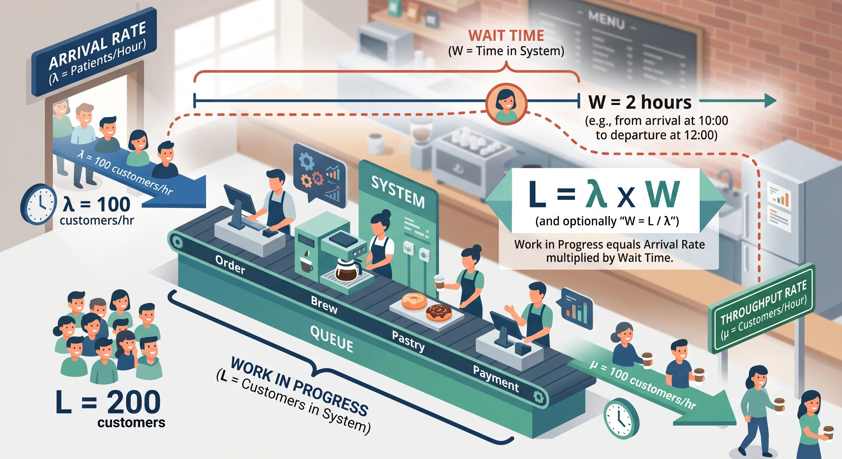
Little’s Law is a fundamental theorem in queueing theory that relates three quantities in any stable system:
L = λ × W
Where:
- L = average number of items in the system (queue length, work-in-progress, etc.)
- λ (lambda) = average arrival rate (items entering the system per unit time)
- W = average time an item spends in the system
Intuition
Imagine a coffee shop. If customers arrive at a rate of 10 per hour (λ), and each customer spends an average of 6 minutes (0.1 hours) in the shop (W), then on average there are:
L = 10 × 0.1 = 1 customer in the shop at any given time.
Why it’s powerful
- It’s remarkably general — it holds for almost any stable system, regardless of the arrival pattern, service time distribution, number of servers, or scheduling policy. It works for coffee shops, call centers, hospital ERs, manufacturing lines, software request queues, and more.
- It requires almost no assumptions — just that the system is “stable” (things aren’t piling up infinitely — the rate in equals the rate out over the long run).
- You can rearrange it to solve for any variable if you know the other two:
- W = L / λ (how long will something wait, given queue size and arrival rate?)
- λ = L / W (what’s the throughput, given average occupancy and time?)
Practical examples
- Software/DevOps: If you have 20 tickets in your backlog (L) and you close tickets at a rate of 5 per day (λ), the average ticket takes W = 20/5 = 4 days to resolve.
- Manufacturing: If a factory has 100 units of work-in-progress and produces 25 units/day, average production time is 4 days.
- Web servers: If a server handles 1000 requests/second and each request takes 200ms on average, there are on average 200 requests “in flight” at any moment.
Common use case: capacity planning
Little’s Law is often used in reverse — if you know how long you want customers to wait (W) and your expected arrival rate (λ), you can figure out how much capacity (L) you need to provision to hit that target.
It’s a simple equation, but it’s foundational because it lets you reason about system performance without needing to know the messy details of how the system works internally — just the rate things come in and how long they stay.