Latency Metrics, From First Principles

systemdesign

1. What latency actually is

Latency is the time elapsed between a request being made and a response being received, for a single unit of work. That’s it. Everything else in this note is about how we measure, summarize, and act on that simple definition at scale.

Three things follow immediately from this definition:

• Latency is a property of a single event, not a system. A system doesn’t “have” one latency — it produces a distribution of latencies, one value per request.
• Latency is directional and boundary-dependent. “Latency” means nothing until you specify where you start the clock and where you stop it (client send → client receive? load balancer in → load balancer out? DB query start → DB query end?). Different boundaries give wildly different numbers for the “same” request.
• Latency is not throughput. Throughput is requests/sec the system processes; latency is how long each one takes. A system can have high throughput and high latency simultaneously (e.g., a batch pipeline), or low throughput and low latency (an idle, fast service). Conflating the two is one of the most common mistakes in performance discussions.

2. Why a single number (“average latency”) is misleading

Latency distributions are almost never symmetric or bell-shaped. They are typically:

• Right-skewed — most requests are fast, a few are very slow (long tail).
• Multi-modal — e.g., one hump for cache hits, another for cache misses; one for warm connections, another for cold TLS handshakes.

Because of skew, the mean (average) is dominated by the tail and tells you almost nothing about the typical user experience, while also being undersensitive to how bad the worst experiences are. Two systems can have the identical average latency while one has a tight distribution and the other has a brutal tail — they are not equivalent, but the average can’t tell them apart.

This is why SRE practice almost universally measures latency using percentiles, not averages.

3. Percentiles: the core building block

The p-th percentile is the value below which p% of observed requests fall.

• p50 (median): half of requests are faster than this. Represents the “typical” experience.
• p90 / p95: the experience of the slower minority. Useful for catching moderate degradation.
• p99: the slow 1%. At scale, 1% is not an edge case — at 1M requests/day, p99 is 10,000 requests.
• p99.9 / p99.99 (“nines”): the deep tail. Matters enormously for systems where a single slow request can stall a user-facing page that’s waiting on many backend calls (fan-out amplifies tail risk — see §6).

Key intuition: as you increase the percentile, you are asking “how bad does it get for an increasingly unlucky subset of users?” SRE work is disproportionately about taming that tail, because the tail is where outages, cascading failures, and the worst user experiences live — even when the median looks perfectly healthy.

A note on the math

Computing exact percentiles from a live, high-volume stream is expensive (it requires knowing the full sorted distribution). In practice systems use:

• Histograms with fixed buckets, accepting some quantization error.
• Approximation algorithms (e.g., t-digest, HDR Histogram) that give accurate tail estimates with bounded memory.
• This matters operationally: a percentile computed by averaging percentiles across hosts is mathematically invalid (percentiles don’t average). You must aggregate the underlying histograms/raw distributions first, then compute the percentile.

4. Latency budgets and composition

End-to-end latency is the sum of latencies across a call chain, plus queuing/wait time at each hop:

total_latency = client_network + LB + app_server_processing
              + downstream_call_1 + downstream_call_2 + ... 
              + serialization + queueing_delay

Two first-principles consequences:

1. Serial dependencies add latency; parallel (fan-out) dependencies add tail risk, not average latency. If a request fans out to N parallel backend calls and waits for all of them, the overall latency is the max of N latencies, not the average. Even if each backend has a clean p99, the probability that at least one of N calls lands in its own tail grows with N. This is why large fan-out systems (search, ad serving, microservice meshes) see tail latency amplification — sometimes called the “tail at scale” problem.
2. A latency budget is an engineering tool: you allocate an acceptable latency ceiling to each component of a request path (e.g., “DNS: 10ms, TLS: 20ms, app: 50ms, DB: 30ms”) so that no single component silently consumes the whole budget. SLOs (below) are usually defined at the boundary the user experiences, while budgets decompose that target internally.

5. SLI, SLO, SLA — the SRE measurement stack

SLO, SLA and SLI

These three terms exist because “latency” alone is not actionable without agreeing on what’s measured, what’s acceptable, and what happens if it isn’t.

• SLI (Service Level Indicator): the actual measurement — e.g., “p99 latency of HTTP 200 responses to /checkout, measured at the load balancer, over a rolling 5-minute window.”
• SLO (Service Level Objective): the target for that SLI — e.g., “p99 latency < 300ms for 99.9% of the trailing 28 days.”
• SLA (Service Level Agreement): the contractual/business consequence if the SLO is missed (refunds, credits) — typically looser than the internal SLO, so you breach your own target before you breach a customer-facing promise.

A precise SLI definition must specify:

• What counts as a valid request (do timeouts count? errored requests? retries — once or every attempt?).
• Where it’s measured (client-side reflects real user experience but is noisier and harder to instrument; server-side is cleaner but can miss network/client-side delay that the user actually feels).
• The aggregation window and percentile.

Sloppy SLI definitions are the single most common cause of “the dashboard says we’re fine but users are complaining” — usually because the SLI is measured server-side while users experience client-side latency, or because it silently excludes errored/timed-out requests (survivorship bias: the requests that failed fastest or hung longest are exactly the ones missing from your “successful request latency” histogram).

6. Error budgets and the role of latency SLOs

If the SLO is “p99 < 300ms for 99.9% of the time,” the error budget is the inverse: the allowed 0.1% of time where you may violate the target. This reframes latency from a vague aspiration (“be fast”) into a finite, spendable resource — you can deliberately trade some of that budget for velocity (e.g., shipping a riskier change) and you have an objective trigger for when to stop and stabilize (budget exhausted).

7. Little’s Law

Introduction

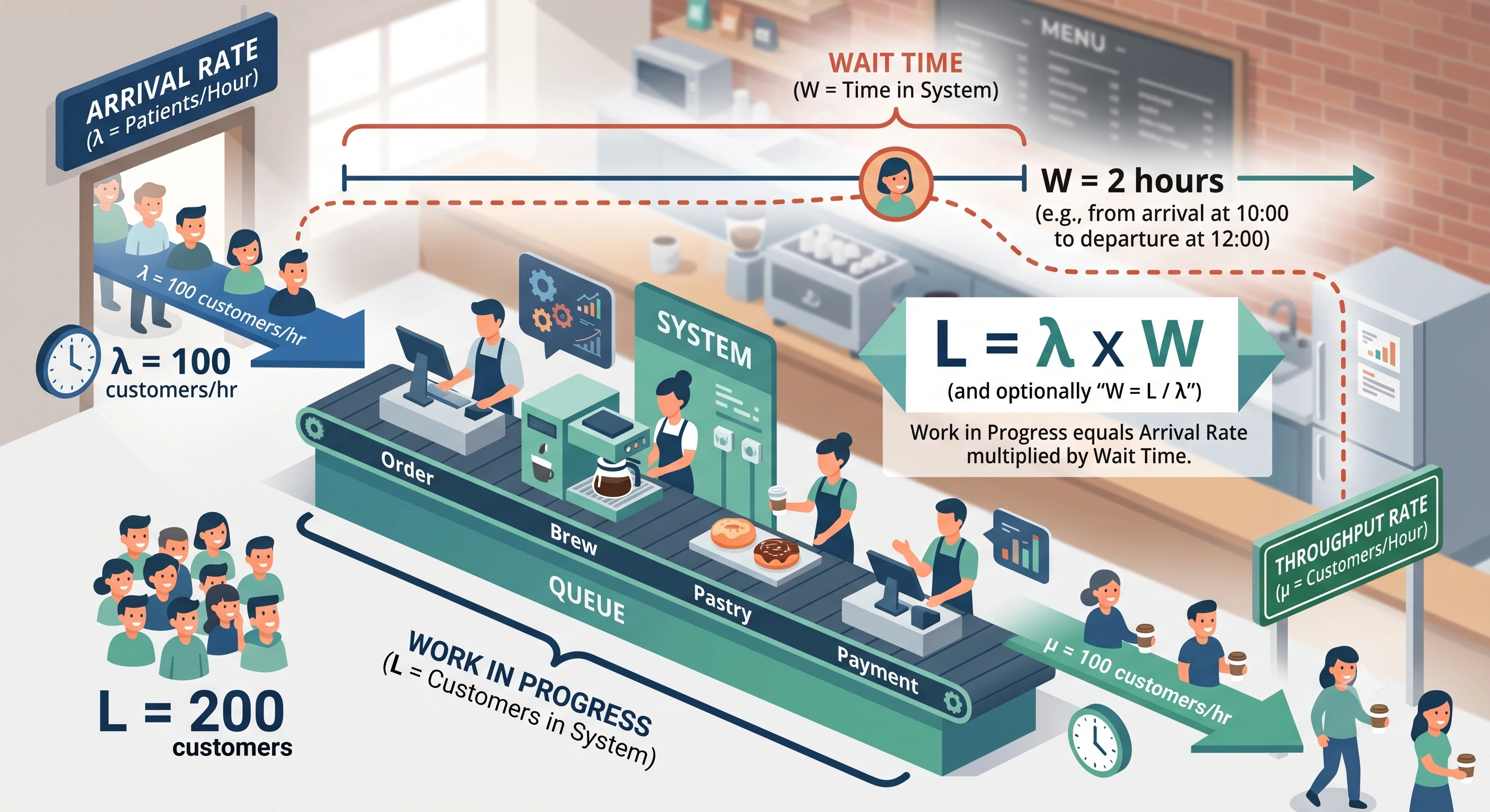
Little’s Law is a fundamental theorem in queueing theory that relates three quantities in any stable system:

L = λ × W

Where:

• L = average number of items in the system (queue length, work-in-progress, etc.)
• λ (lambda) = average arrival rate (items entering the system per unit time)
• W = average time an item spends in the system
  

Link to original

8. Practical pitfalls (first-principles traps people fall into)

• Averaging percentiles across machines/services. Invalid — percentiles aren’t linear, so avg(p99_host1, p99_host2, ...) ≠ true p99 across hosts. Aggregate raw distributions/histograms first.
• Excluding errors/timeouts from the latency SLI. A request that times out at 30s “doesn’t count” toward your p99 — but the user absolutely experienced it. This artificially inflates apparent performance.
• Confusing client-perceived latency with server-measured latency. Server-side measurement misses queueing at the load balancer, DNS, TLS handshake, and network transit — all real to the user.
• Ignoring retries. If a client retries failed/slow requests, “per-attempt” latency can look fine while “per-logical-request” (including retries) latency is poor. Decide explicitly which you’re measuring.
• Treating throughput and latency as independent. Per Little’s Law, they aren’t — load testing should report latency as a function of load, not as a single number at one traffic level.
• Picking a percentile that’s too low to catch the problem you care about. If 1 in 200 requests triggers a customer complaint, p99 (1 in 100) is coarse enough to catch it on average, but p95 won’t.

9. Summary: the mental model

1. Latency is per-request; a system produces a distribution.
2. Distributions are skewed — use percentiles, not averages, and pick the percentile that matches the harm you’re trying to detect.
3. Tail latency compounds under fan-out and high load (Little’s Law) — this is where outages live.
4. Turn the distribution into something actionable via SLI → SLO → error budget, defined precisely (boundary, inclusion criteria, window).
5. Always ask: measured where, including what, relative to how much load? — those three questions resolve almost every latency-metric disagreement.