Small Language Model

llm agents ai slm

Based on the book Domain-Specific Small Language Models: Efficient AI for Local Deployment by Guglielmo Iozzia.

Introduction

LLMs have transformed artificial intelligence by enabling applications such as text generation, code generation, question answering, and intelligent assistants. However, these models often require significant computational resources, high deployment costs, and access to powerful hardware. They can also raise concerns about data privacy, security, and control.

Small Language Models (SLMs) offer an alternative. By using fewer parameters and focusing on specific domains or tasks, SLMs can deliver useful AI capabilities with lower memory requirements and reduced computational costs. They are particularly suitable for local deployment on laptops, CPUs, mobile devices, and private infrastructure.

Tuning for a Specific Domain

Three main approaches:

1. RAG — Extend model knowledge using external data.
2. Fine-Tuning — Update model weights using task-specific training data.
3. LoRA — Efficiently adapt models by training a small number of additional parameters.

Core Idea

RAG provides knowledge. Fine-tuning develops task-specific capabilities. LoRA reduces the cost of model adaptation.

The best strategy depends on the use case, data availability, computational resources, and accuracy requirements.

Data Preparation

Data preparation is the first step in customizing a pretrained Transformer model.
Different architectures require different training formats.

Model	Data Format	Use Case
BERT	Text + Label	Classification
GPT-2	Prompt + Completion	Text Generation
RAG	Documents + Embeddings	Knowledge Retrieval

BERT Data Preparation

BERT is an encoder-based Transformer commonly used for text understanding tasks.

Workflow:

1. Collect labeled training data.
2. Tokenize text with the BERT tokenizer.
3. Apply padding and truncation.
4. Convert tokens into numerical IDs.
5. Create attention masks.
6. Split data into training and validation sets.
7. Prepare PyTorch DataLoaders.

Special tokens:

• [CLS] — Marks the beginning of a sequence.
• [SEP] — Separates segments.
• [PAD] — Pads shorter sequences.

1.2 GPT Data Preparation

GPT is a decoder-based Transformer designed for text generation.

Training data consists of input-output pairs.

Example:

Input:
Summarize this technical document.

Target:
A short summary of the document.

The model learns to generate the target sequence from the input context.

1.3 Data Preparation for RAG

RAG requires converting external documents into searchable representations.

Workflow:

1. Collect domain-specific documents.

2. Prepare text for embedding.

3. Convert text into vector embeddings.

4. Store embeddings in a vector index.

5. Perform similarity searches to retrieve relevant information.

The chapter demonstrates FAISS for indexing and searching vector embeddings.

Retrieval-Augmented Generation (Section 2.2)

RAG combines information retrieval with language generation.

Instead of updating model weights, it supplies relevant external knowledge during inference.

RAG Workflow

1. User submits a query.

2. The retrieval system searches an external knowledge source.

3. Relevant information is retrieved.

4. The query and retrieved context are passed to the language model.

5. The model generates an answer using the supplied context.

Advantages

• No model retraining required.

• Supports frequently changing information.

• Can improve factual grounding.

• Enables source traceability.

• Useful for private enterprise knowledge.

Limitations

• Depends on retrieval quality.

• Requires indexing and search infrastructure.

• Adds retrieval overhead.

• Cannot reliably compensate for missing model capabilities.

Example — Enterprise Knowledge Assistant

An organization stores internal policies and technical manuals in a searchable knowledge base.

A user asks: “What is our procedure for handling customer data?”

RAG retrieves the relevant policy and passes it to the model, which generates an answer grounded in that document.

3. Fine-Tuning (Section 2.3)

Fine-tuning further trains a pretrained language model using a smaller task-specific dataset.

Unlike RAG, fine-tuning updates the model’s parameters.

Fine-Tuning Workflow

1. Select a pretrained foundation model.

2. Prepare domain-specific labeled data.

3. Tokenize and preprocess the dataset.

4. Divide the dataset into training and evaluation sets.

5. Train the model.

6. Evaluate its task-specific performance.

Example from the Book

The chapter uses DistilBERT for extractive question answering.

Training samples contain:

• question — User question.

• context — Relevant source text.

• answers — Answer text and its position in the context.

Advantages

• Learns specialized terminology and patterns.

• Can improve task-specific performance.

• Adapts model behavior to specific domains.

• Useful for structured or specialized generation.

Limitations

• Requires task-specific datasets.

• More computationally expensive than RAG-based customization.

• Requires machine learning expertise.

• May introduce overfitting or reduce existing capabilities.

Key Learning

Fine-tuning is useful when a model needs to learn a specialized task or representation, rather than simply retrieve additional facts.

4. LoRA — Low-Rank Adaptation (Section 2.4)

LoRA is a Parameter-Efficient Fine-Tuning technique that reduces the number of trainable parameters.

How LoRA Works

Traditional Fine-Tuning

• Updates all pretrained model parameters.
• Requires more compute and memory.

LoRA

• Freezes the original model weights.
• Introduces small trainable low-rank matrices.
• Trains these matrices instead of the full model.
• Reduces training resource requirements.

Example from the Book

Model: google/flan-t5-small

Dataset: SAMSum

Task: Dialogue summarization.

LoRA configuration:

• Rank (r): 16
• Alpha: 32
• Dropout: 0.05
• Target modules: Query and Value projections

Result:

• Trainable parameters: 688,128
• Percentage of model trained: approximately 0.89%

This demonstrates that only a small fraction of parameters need to be trained for model adaptation.

Other PEFT Techniques

• Prefix tuning
• Prompt tuning
• P-tuning
• AdaLoRA
• LoftQ

Key Learning

LoRA makes domain-specific model adaptation more accessible when training resources are limited.

It is especially valuable when customizing pretrained SLMs.

5. RAG vs Fine-Tuning vs LoRA (Section 2.5)

Criteria	RAG	Fine-Tuning	LoRA
Model weights updated	No	All	Adapter weights
Model training needed	No	Yes	Yes
Training cost	None	High	Lower
Dynamic knowledge	Excellent	Requires updates	Requires updates
Specialized task learning	Limited	Strong potential	Strong potential
Source traceability	Strong	Limited	Limited
Hardware requirements	Retrieval + inference	High	Lower
Typical use case	Knowledge retrieval	Specialized tasks	Efficient adaptation

How Do You Choose?

Use RAG when:

• Information changes frequently.

• You need answers grounded in external documents.

• Source traceability is important.

Use Fine-Tuning when:

• The model needs to learn specialized patterns.

• A domain requires structured or complex generation.

• Sufficient quality training data is available.

Use LoRA when:

• Fine-tuning is useful but computational resources are limited.

• You want an efficient adaptation of an existing model.

• You need reusable task-specific adapters.

Important Consideration

RAG is not always cheaper than fine-tuning in the long run. Large retrieval systems require infrastructure, maintenance, and data pipelines.

Fine-tuning and RAG can also complement each other.

ONNX - Open Neural Network Exchange

1. What is ONNX?

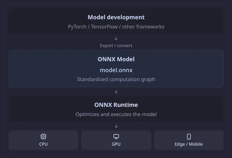
ONNX (Open Neural Network Exchange) is an open standard for representing machine learning models so they can run across different frameworks, operating systems, and hardware platforms.

Think of ONNX as a universal model format.

For example, you can:

• Train a model using PyTorch.
• Convert it into ONNX format.
• Optimize it for faster inference.
• Run it on a CPU, GPU, or supported edge device using ONNX Runtime.

Key idea: ONNX separates how a model is developed from how it is deployed.

2. How ONNX works

3. ONNX has two important parts

Component	Purpose
ONNX format	Stores a model as a standardized computation graph
ONNX Runtime (ORT)	Executes that model efficiently on supported hardware

ONNX Format

An ONNX model is represented as a computational graph containing operators and tensors.

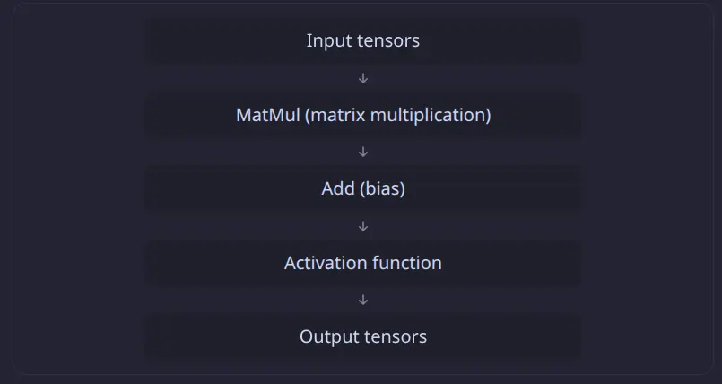
Each operation is represented as a node, and the connections between nodes carry tensors containing numerical data.

Common operators include MatMul, Add, Softmax, LayerNormalization, and Reshape.

ONNX Runtime

ONNX Runtime is the engine that runs the graph. It can optimize computations and select hardware-specific execution providers, such as:

• CPU Execution Provider
• CUDA Execution Provider for NVIDIA GPUs
• TensorRT Execution Provider
• OpenVINO Execution Provider
• DirectML Execution Provider

Hardware availability and support determine which provider can be used.

4. Why is ONNX important for small language models?

The book emphasizes three main benefits.

1. Portability: A model trained using PyTorch can be exported to ONNX and deployed without requiring the original training framework for inference.

2. Performance optimization: ONNX Runtime supports graph transformations such as operator fusion, constant folding, and other optimizations. These can reduce inference overhead.

3. Hardware flexibility: ONNX models can execute on CPUs and supported accelerators, making them useful for local servers, laptops, and edge devices.

ONNX does not guarantee that every model will become faster. Performance must be benchmarked on the target hardware.

5. Practical Python example

Suppose you already have an exported file named model.onnx.

Install the CPU runtime:

pip install onnx onnxruntime

Run inference:

import onnxruntime as ort
import numpy as np
 
# Load the ONNX model
session = ort.InferenceSession(
    "model.onnx",
    providers=["CPUExecutionProvider"]
)
 
# Inspect input and output names
input_name = session.get_inputs()[0].name
output_name = session.get_outputs()[0].name
 
# Example input for a compatible numerical model
input_data = np.array(
    [[2.0, 4.0, 6.0, 8.0]],
    dtype=np.float32
)
 
# Run inference
result = session.run(
    [output_name],
    {input_name: input_data}
)
 
print(result[0])

This follows the inference workflow presented in Chapter 5, Section 5.3. The example input shape and data type must match the actual ONNX model; a language model generally requires token IDs, attention masks, and sometimes additional inputs.

6. ONNX and quantization

One important distinction: ONNX is not itself a quantization technique.

However, ONNX models can be quantized to lower-precision numerical formats.

Precision	Typical storage per weight
FP32	4 bytes
FP16	2 bytes
INT8	1 byte
INT4	0.5 bytes

For example, a model containing 1 billion parameters would require approximately 4 GB just for FP32 weights, versus 1 GB for INT8 weights, ignoring quantization metadata and other runtime memory.

Quantization reduces storage and memory requirements but can affect output accuracy. The book expands on this in Chapter 6.

8. When should you use ONNX?

Scenario	Is ONNX useful?
Deploying a PyTorch model on a CPU server	Yes
Optimizing BERT inference	Yes
Deploying models across different hardware	Yes
Running an AI model on an edge device	Often
Training a model from scratch	Usually not the primary tool
Running a local chatbot with Ollama	Usually not necessary

ONNX is particularly valuable when you need control over model execution and optimization. If your main objective is simply to run a local chatbot, a dedicated runtime such as Ollama may be easier.

Chapter 5 takeaway: ONNX provides a standard way to represent and optimize machine learning models, while ONNX Runtime makes them executable across diverse hardware environments.

Recommended next topic: Understand the relationship between ONNX graph optimization, ONNX Runtime execution providers, and quantization. These are the most valuable concepts for efficient local SLM deployment.